Introduction Transformer Model from Math Perspective

Transformer

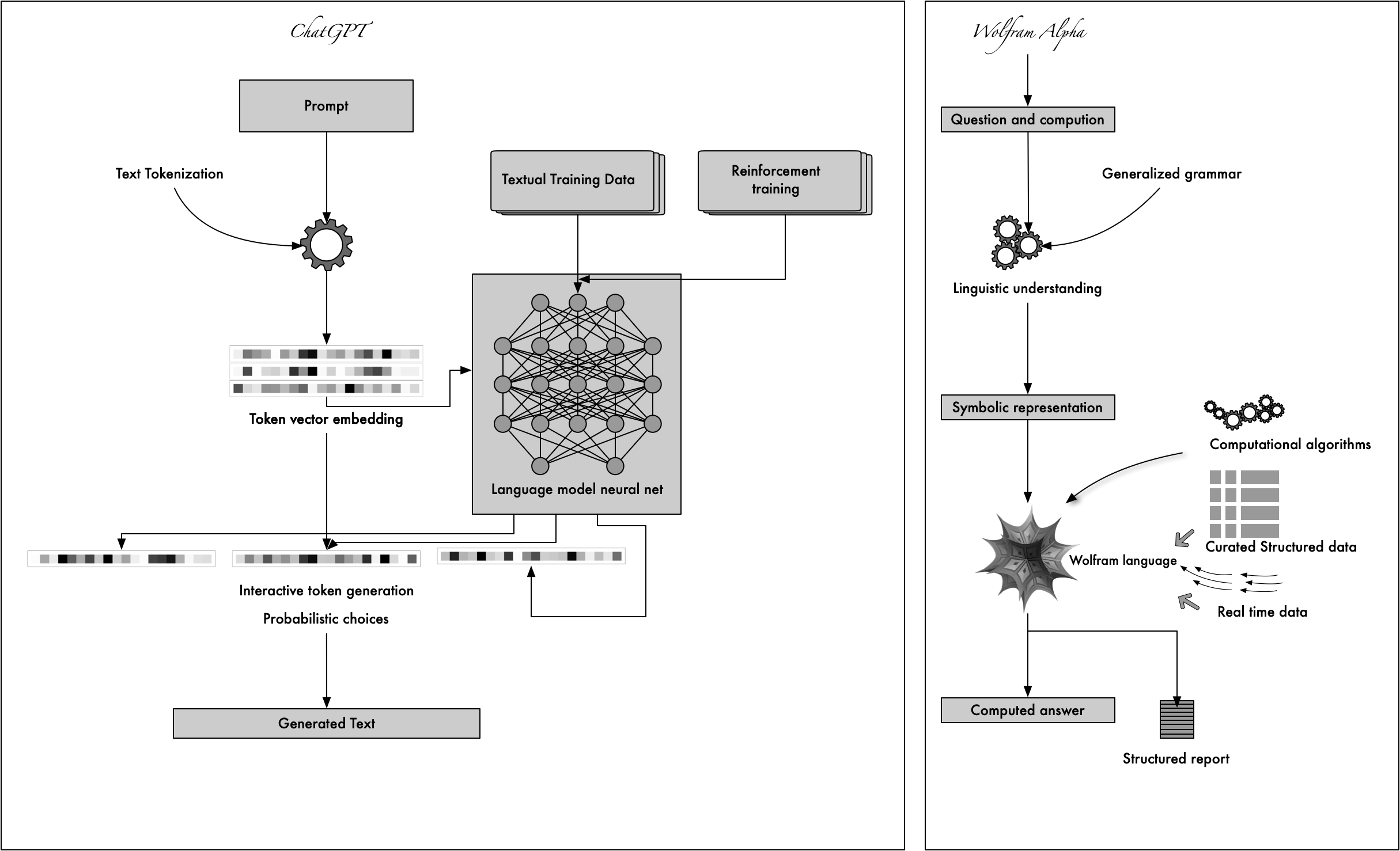
Last year when OpenAI published ChatGPT, the large language model (LLM) making waves in AI community. why chatgpt works so well? can we understand the internal of GPT?

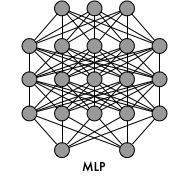
Deep learning neural network like a black box, we can only know the result from it, but can’t understand the data process in it’s internal. for example deign a MLP neural neural work, does the number of layers need 5 or 6 or more to get the more accurate answers? sorry no theory to prove that because of the deep neural network can’t explained. so turn to ChatGPT, we will dive into the chatgpt internal to understand it’s operational mechanism.

Tansformer is the basic architecture of GPT, so the first things first, we will use mathematics language to understand the transformer model.

The Transformer model has four parts:

Embedding
Encoder
Decoder
Softmax

we will use Wolfram language and mathematics to struct these four parts.

EmbeddingBlock

Tokenizer

when we put text sequences to transformer net, we need to convert the texts string type into numericArray type, but what methods can we convert language text to numericArray. The answer is “SubWordTokens” method. Suppose, we have a big dictionary book which have all meta tokens that represent all meta words. we use “vocabulary” to representation of this dictionary book. so we define the vocabulary size is N, the sequences of language text can be represent some points set in vocabulary N dimensions space. echo vocabulary element is assigned a uniq index:

\text{[N] = } \left\{1,2,\text{...},N_v\right\}

A piece of text is represented as a sequence of indices , we call it as Token IDs, corresponding to its subwords. In vocabulary there are three special tokens:

mask token (used in masked language modeling)
bos token (represent beginning of sequence)
eos token (represent end of sequence)

For example:

Wolfram

vocabulary = NetExtract[ResourceFunction["GPTTokenizer"][], "Tokens"];
voca = NetExtract[ResourceFunction["GPTTokenizer"][], "Tokens"];
(* tokenizer encoder: convert text strings to tokenIDs *)
netTextEncoder = ResourceFunction["GPTTokenizer"][]

(* tokenizer decoder: convert tokenIDs to string sequence*)
netTextDecoder = 
 NetDecoder[{"Class", 
   NetExtract[ResourceFunction["GPTTokenizer"][], "Tokens"]}]

seq = netTextEncoder["what is transformer language model"]
(* represent sequence tokenIDs *)
(* output is {10920, 319, 47386, 3304, 2747}*)

(* convert tokenIDs to sequence *)

(* map tokenIDs to vector of vocabulary space *)
tokenids = Map[UnitVector[Length@voca, #] &, seq] 

StringReplace[StringJoin@Map[netTextDecoder[#] &, tokenids], 
 "Ġ" -> " "]
(* output is "what is transformer language model" *)
(* Ġ represent whitespace *)

Now we can represent string sequences as tokenIDs that easier to feed into our neural network.

Embedding

The embedding layer converts an input sequence of tokens into a sequence of embedding vectors, we call it as Context.

V represent vocabulary
N represent vocabulary index
e represent embedding Token
W represent matrix
W(All, i) represent the i column of the matrix
W(i, All) represent the i row of the matrix
t represent index of token in a sequence
l represent length of token sequence

Token Embedding Algorithm:

\text{Input} \text{: v $\in $ V} \left[N_v\right] \text{, } a \;\text{token} \; \text{ID} \\ \text{Output} \text{: e $\in $ } \mathbb{R}^{d_e}, \text {the}\, \text {vector} \,\text{of}\, \text{representation} \, \text {of}\, \text{the} \,\text{token} \\ \text{Parameters} \text{: } W_e \text{$\in $ } \mathbb{R}^{d_e * N_v} \text{, the token embedding matrix } \\ \text{Return} \text{: e = } W_e(\text{All},v)

Because transformer mode only use forward network, no recurrent or backward network, the model essentially can not know the positional of token. so we need feed some token positional information into the network, we call it positional embedding.

Positional hardcode Embedding Algorithm:

W_p \text{ : $\mathbb{N}$ $\rightarrow $ } \mathbb{R}^{d_e} \text{, use equations:} \\ W_p \text{[2i - 1, t] = } \sin \left(\frac{t}{\ell _{\max }^{\frac{2 i}{d_e}}}\right) \\ W_p \text{[2i , t] = } \cos \left(\frac{t}{\ell _{\max }^{\frac{2 i}{d_e}}}\right) \\ \text{0 $<$ i $\leq $ } \frac{d_e}{2} \\ \text{For the t-} \text{th} \text{ token , the embedding is:} \\ \pmb{\text{e = }} W_e(\text{All},x(t))+W_p(\text{All},t)

Wolfram

(* learned positional embeding *)
embedding[embedDim_, vocabulary_] := 
 NetInitialize@NetGraph@FunctionLayer[
    (* learned position embeding  *)
    Block[{emb1, emb2, posembed},
      emb1 = EmbeddingLayer[embedDim][#Input];
      posembed = SequenceIndicesLayer[embedDim][#Input];
      emb2 = EmbeddingLayer[embedDim][posembed];
      emb1 + emb2 ] &,
    "Input" -> {"Varying", NetEncoder[{"Class", vocabulary}]}]

token embedding + trained able positional embedding net graph, (context dimension is 128):

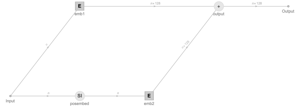
For example, we set embedding dimension is 64:

Wolfram

ArrayPlot[
 embedding[64, voca][
  StringSplit["what is transformer language model"]]]

“what is transformer language model” sequence will be represented by a numericArray. every row representation one word. black, white, grayscale squares mean the value of embedding output, the dimensions of output is (5, 64)

Wolfram

(* hard code positional embeding *)
coeffsPositionalEncoding[embedDim_] := 
  NetMapOperator[
   LinearLayer[embedDim/2,
    "Weights" -> 
     List /@ Table[1./10000.^(2 i/embedDim ), {i, embedDim/2}],
    "Biases" -> None, "Input" -> "Integer",
    LearningRateMultipliers -> 0
    ]
   ];

embeddingSinusoidal[embedDim_, vocabulary_,dropout_ : 0.1] := NetInitialize@NetGraph[
   <|
    "sequenceLength" -> SequenceIndicesLayer[],
    "coeffs" -> coeffsPositionalEncoding[embedDim],
    "sin" -> ElementwiseLayer[Sin],
    "cos" -> ElementwiseLayer[Cos],
    "catenate" -> CatenateLayer[2],
    "+" -> ThreadingLayer[Plus],
    "dropout" -> DropoutLayer[dropout],
    "embeddingTokenID" -> 
     EmbeddingLayer[embedDim, 
      "Input" -> {"Varying",  NetEncoder[{"Class", vocabulary}]}]
    |>,
   {
    NetPort["Input"] -> 
     "sequenceLength" ->  
      "coeffs" -> {"sin", "cos"} -> "catenate" ->  "+" -> "dropout",
    NetPort["Input"] -> "embeddingTokenID" -> "+"}
   ]

Positional Learned Embedding Algorithm:

\text{Input} \text{: $\ell $ $\in $ } \left[\ell _{\max }\right] \text{, position a token in the sequence} \\ \text{Output} \text{: } e_p \text{ $\in $ } \mathbb{R}^{d_e}, \text {the vector representation of the position} \\ \text{Parameters} \text{: } W_p \text{$\in $ } \mathbb{R}^{d_e * \ell _{\max }}, \text {the positional embedding matrix} \\ \text{Return} \text{: e = } W_p(\text{All},\ell )

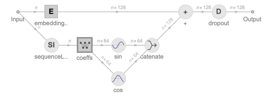
token embedding + hard code positional embedding net graph (context dimension is 128):

Wolfram

ArrayPlot[
 embeddingSinusoidal[64, voca][
  StringSplit["what is transformer language model"]]]

we can see that the squares of the rows are easy to distinguish, just like the learned embedding.

now, we combine all the functions into embeddingBlock:

Wolfram

Options[embeddingBlock] = {"depth" -> None, "voca" -> None, 
   "hardCode" -> False};
embeddingBlock[OptionsPattern[]] := Block[
  {embedding, embeddingSinusoidal, posencoding, 
   embedDim = OptionValue["depth"], 
   vocabulary = OptionValue["voca"],
   posWeightHardCode = OptionValue["hardCode"]},
  
  posencoding[embedDim_] := NetMapOperator[
    LinearLayer[embedDim/2,
     "Weights" -> 
      List /@ Table[1./10000.^(2 i/embedDim ), {i, embedDim/2}],
     "Biases" -> None, "Input" -> "Integer",
     LearningRateMultipliers -> 0
     ]
    ];
  
  embedding[embedDim_, vocabulary_] := 
   NetInitialize@NetGraph@FunctionLayer[
      (* learned position embeding  *)
      Block[{emb1, emb2, posembed, add, dropout},
        emb1 = EmbeddingLayer[embedDim][#Input];
        posembed = SequenceIndicesLayer[embedDim][#Input];
        emb2 = EmbeddingLayer[embedDim][posembed];
        add = emb1 + emb2;
        dropout = DropoutLayer[0.1][add]] &,
      "Input" -> {"Varying", NetEncoder[{"Class", vocabulary}]}];
  
  embeddingSinusoidal[embedDim_, vocabulary_,  dropout_ : 0.1] := 
   NetInitialize@NetGraph[
     <|
      "sequenceLength" -> SequenceIndicesLayer[],
      "coeffs" -> posencoding[embedDim],
      "sin" -> ElementwiseLayer[Sin],
      "cos" -> ElementwiseLayer[Cos],
      "catenate" -> CatenateLayer[2],
      "+" -> ThreadingLayer[Plus],
      "dropout" -> DropoutLayer[dropout],
      "embeddingTokenID" -> 
       EmbeddingLayer[embedDim, 
        "Input" -> {"Varying",  NetEncoder[{"Class", vocabulary}]}]
      |>,
     {
      NetPort["Input"] -> 
       "sequenceLength" ->  
        "coeffs" -> {"sin", "cos"} -> 
          "catenate" ->  "+" -> "dropout",
      NetPort["Input"] -> "embeddingTokenID" -> "+"}
     ];
  If[posWeightHardCode,
   embeddingSinusoidal[embedDim, vocabulary],
   embedding[embedDim, vocabulary]]
  ]
  
embeddingBlock["depth" -> 128, "voca" -> voca, "hardCode" -> False]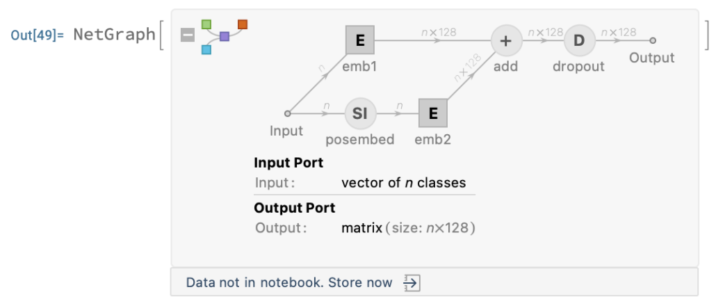

EncoderBlock

SelfAttention Unit

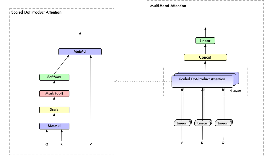
Attention is the main architectural component of transformer. It enables a neural network to make use of context information for predicting the current token.

Basic Single Query Attention Algorithm:

\text{Input} \text{: e $\in $ } \mathbb{R}^{d_{\text{in}}} \text{ ,} \text {vector represent of the current token, Q in figure-2} \\ \text{Input} \text{: } e_t \text{ $\in $ } \mathbb{R}^{d_{\text{in}}} \text{, } \text {vector represent of context tokens, K, V in figure-2} \\ \text{Output} \text{: } \tilde{v} \text{$\in $ } \mathbb{R}^{d_{\text{out}}} , \text {vector representation of the token and context combined} \\ \text{Parameters} \text{: } W_q,W_k \text{$\in $ } \mathbb{R}^{d_{\text{atten}} * d_{\text{in}}} \text{, } b_q,b_k \text{$\in $ } \mathbb{R}^{d_{\text{atten}}} \text { the query and key linear projections} \\ \text{Parameters} \text{: } W_v \text{ $\in $ } \mathbb{R}^{d_{\text{in}} *d_{\text{out}}} \text{, } b_v \text{$\in $ } \mathbb{R}^{d_{\text{out}}}, \text {the value linear projection}

Attention Pseudo Code: (UnMasked SelfAttention)

\text{q $\leftarrow $ } e W_q \text{ + } b_q \\ \text{$\forall $t: } k_t \text{$\leftarrow $ } b_k+e_t W_k \\ \text{$\forall $t: } v_t \text{$\leftarrow $ } b_v+e_t W_v \\ \text{$\forall $t: } \alpha _t \text{= } \frac{e^{\frac{k_t q^T}{\sqrt{d_{\text{atten}}}}}}{\sum _u e^{\frac{k_u q^T}{\sqrt{d_{\text{atten}}}}}} = \text{Attention(Q, K, V) } = \text{softmax}\left(\frac{Q K^T}{\sqrt{d_k}} \right) \text V \\ \tilde{v} \text{ = } \sum _{t=1}^T \alpha _t v_t

Q, K, V are linear processor, Q maps current token to a query vector, K maps current context to a key vector, V maps current context to a value vector
Q and K matrix multiplication, interpreted as the degree to which token t is important for predicting the current token q
softmax combine with V use matrix multiplication

Masked SelfAttention Algorithm:

\text{Input: X $\in $ } \mathbb{R}^{d_x * \ell _x}, Z \text{$\in $ } \mathbb{R}^{d_z * \ell _z}, \text {vector representations of primary and context sequence.} \\ \text{Output: } \tilde{V} \text{ $\in $ } \mathbb{R}^{d_{\text{out}} * \ell _x} \text {updated representations of tokens in X, folding in information from tokens in Z} \\ \text{Parameters: } W'_{\text{qkv}} \text{ consisting of:} \\ \text{$\quad \quad |$ } W_q \text{$\in $ } \mathbb{R}^{d_{\text{atten}} * d_x} \text{, } b_q \text{ $\in $ } \mathbb{R}^{d_{\text{atten}}} \\ \text{$\quad \quad |$ } W_k \text{$\in $ } \mathbb{R}^{d_{\text{atten}}* d_z} \text{, } b_k \text{ $\in $ } \mathbb{R}^{d_{\text{atten}}} \\ \text{$\quad \quad |$ } W_v \text{$\in $ } \mathbb{R}^{d_{\text{out}}* d_z} \text{, } b_v \text{ $\in $ } \mathbb{R}^{d_{\text{out}}} \\ \text{Hyperparameters: Mask $\in $ } \{0,1\}^{\ell _x \ell _z} \\ \text{Mask}\left[t_z,t_x\right] \text{=1}, \text {for bidirectional attention} \\ \text{Mask}\left[t_z,t_x\right] \text{ = 0,} \text {for unidirectional attention when } t_z < t_x

Masked SelfAttention pseudo code:

\text{Q $\leftarrow $ } 1^T b_q+X W_q \text{ [[Query $\in $ } \mathbb{R}^{d_{\text{atten}} * \ell _x} \text{]]} \\ \text{K $\leftarrow $ } 1^T b_k+Z W_k \text{ [[Key $\in $ } \mathbb{R}^{d_{\text{atten}} * \ell _z} \text{]]} \\ \text{V $\leftarrow $ } 1^T b_v+Z W_v \text{ [[Value $\in $ } \mathbb{R}^{d_{\text{atten}}* \ell _z} \text{]]} \\ \text{S $\leftarrow $ } Q K^T \text{ [[Score $\in $ } \mathbb{R}^{\ell _x * \ell _z} \text{]]} \\ \text{For All } t_z, t_x, \text{if} \text{ not } \text{Mask}\left[t_z,t_x\right], \text{then } S\left[t_z\right. \text{, } t_x \text{] $\leftarrow $ -$\infty $} \\ \tilde{V} \text{ = V $\cdot $ softmax(S/} \sqrt{d_{\text{attn}}} )

classes of selfAttentions:

Unmasked SelfAttention
- Apply attention to each token, the the context k has all sequence tokens
Masked SelfAttention
- Apply attention to each token, but the context has only preceding tokens, using causal mask ensures that each location only has access to the location that come before it, this version can be used for online prediction.
Cross Attention
- often used in sequence to sequence task, give two sequences of token representations X,Z, use Z as context sequence, and set mask=1, the output V’s length as same as input X, but the Z’s length can be different with X’s length.

\text{MultiHead(Q, K, V) = } \text{Concat}\left(\text{head}_1,\text{head}_2,\text{...}.,\text{head}_n\right. ) W^O

Multi head self attention Algorithm

the structure of MHA is same as Basic Single Query Attention, but it has multiple attention heads, with separate learnable parameters. (figure-2)

\text{Input} \text{: X $\in $ } \mathbb{R}^{d_x * \ell _x} \text{, Z $\in $ } \mathbb{R}^{d_z * \ell _z} \text {vector representation of primary and context sequence} \\ \text{output} \text{: } \tilde{v} \text{$\in $ } \mathbb{R}^{d_{\text{out}} * \ell _x}\text {updated representation of tokens in X, folding in information from tokens in Z} \\ \text {Hyperparameters: H, number of attention heads} \\ \text{HyperParameters: } \text{Mask $\in $ } \{0,1\}^{\ell _x * \ell _z} \\ \text{Parameters} \text{: } W' \text{consisting} \text{of}: \\ \text{For h $\in $ [H], } \left(W'\right)_{\text{qkv}}^h \text{ consisting of :} \\ \text{$\quad \quad |$ } W_q^h \text{$\in $ } \mathbb{R}^{d_{\text{atten}}* d_x} \text{, } b_q^h \text{ $\in $ } \mathbb{R}^{d_{\text{atten}}} \\ \text{$\quad \quad |$ } W_k^h \text{$\in $ } \mathbb{R}^{d_{\text{atten}}* d_z} \text{, } b_k^h \text{ $\in $ } \mathbb{R}^{d_{\text{atten}}} \\ \text{$\quad \quad |$ } W_v^h \text{$\in $ } \mathbb{R}^{d_{\text{mid}}*d_z} \text{, } b_v^h \text{ $\in $ } \mathbb{R}^{d_{\text{mid}}} \\ W_O \text{ $\in $ } \mathbb{R}^{d_{\text{out}} *\text{Hd}_{\text{mid}}} \text{, } b_O \text{$\in $ } \mathbb{R}^{d_{\text{out}}}

Multi head self attention Pseudo Code

\text{For h $\in $ [H]} \\ Y^h \text{ $\leftarrow $ Attention(X, Z$|$} \left(W'\right)_{\text{qkv}}^h \text{, Mask)} \\ Y \text{ $\leftarrow $ } \left[Y^1;Y^2;Y^3,\text{Null}\ldots \right. \text{;, } \left.Y^H\right] \\ \tilde{V} \text{ = } Y W_O \text{ + } I^T b_O

Wolfram

selfAttentionBlock[embedDim_, heads_, masking_ : None] := 
 NetInitialize[
  NetGraph[
   FunctionLayer[
    Block[{keys, queries, values, seq, attention, merge},
      (* pre layer normalization*)
      seq = 
       NormalizationLayer[2 ;;, "Same", 
         "Epsilon" -> 0.0001 ][#Input];
      keys = NetMapOperator[{heads, embedDim/heads}][seq];
      queries = NetMapOperator[{heads, embedDim/heads}][seq];
      values = NetMapOperator[{heads, embedDim/heads}][seq];
      attention = 
       AttentionLayer["Dot", "MultiHead" -> True, "Mask" -> masking, 
         "ScoreRescaling" -> "DimensionSqrt"][<|"Key" -> keys, 
         "Query" -> queries, "Value" -> values|>];
      merge = NetMapOperator[embedDim][attention];
      seq = DropoutLayer[0.1][merge];
      seq = seq + #Input
      ] &, "Input" -> {"Varying", embedDim}
    ]
   ]
  ]

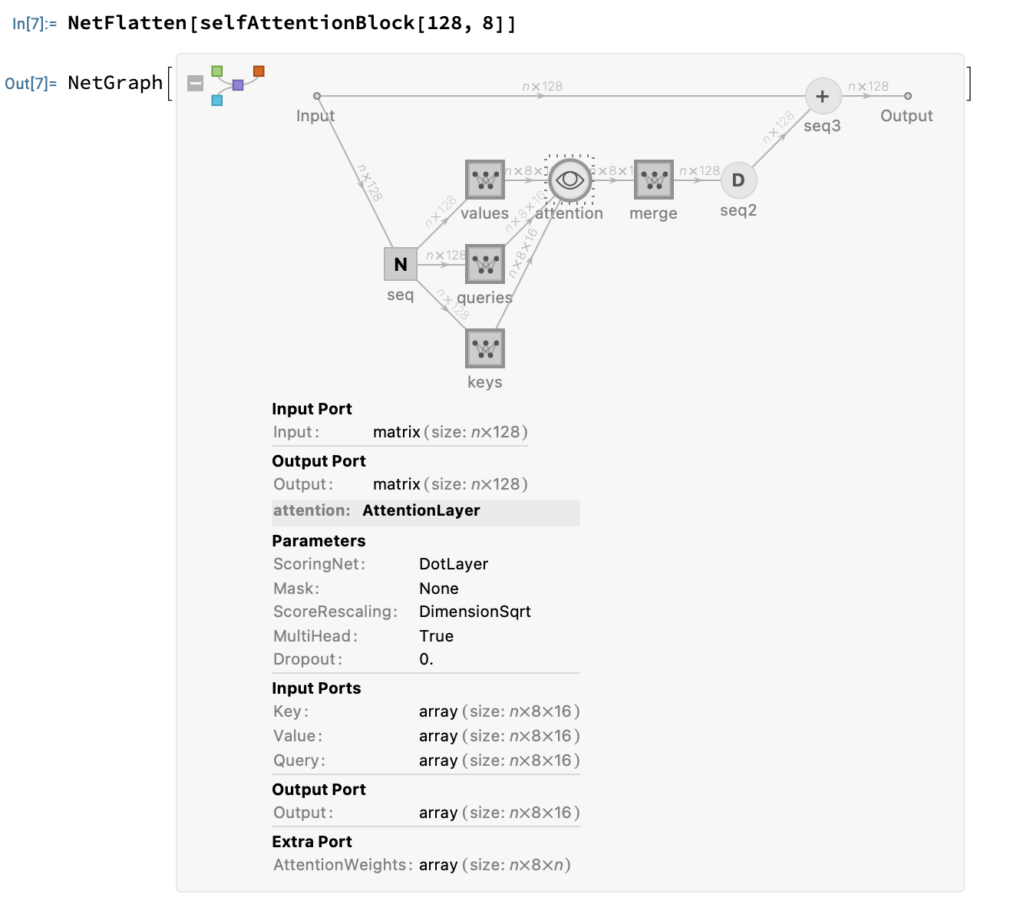
if the model’s embedding dimension is 128, and use 8 attention heads, then the key’s query’s and value’s dimension is n * 8 * 16, in the selfAttentionBlock we use linearLayer to merge all attention heads to n * 128 dimension.

Feed Forward Network

Wolfram

feedForwardBlock[embedDim_] := NetInitialize[
  NetGraph[
   FunctionLayer[
    Block[{seq},
      seq = 
       NormalizationLayer[2 ;;, "Same", "Epsilon" -> 0.0001][#Input];
      seq = NetMapOperator[4 embedDim][seq];
      seq = ElementwiseLayer["GELU"][seq];
      seq = NetMapOperator[embedDim][seq];
      seq = DropoutLayer[0.1][seq];
      seq = seq + #Input
      ] &,
    "Input" -> {"Varying", embedDim}
    ]
   ]
  ]
  
Information[feedForwardBlock[128], "SummaryGraphic"]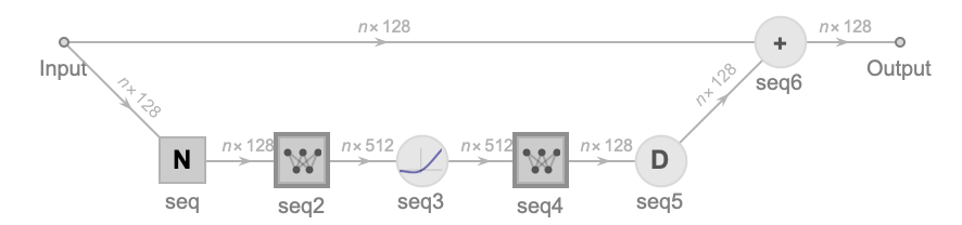

In feed forward network, there are two linearLayers, the first one’s output dimension is n*512, then use a “GELU” activation, after that, the data will be process by another one which the output dimension is n * 128. Notice that in the attention and feedForward network, we use pre layer normalization arrangements, this also same in decoder network.

Decoder

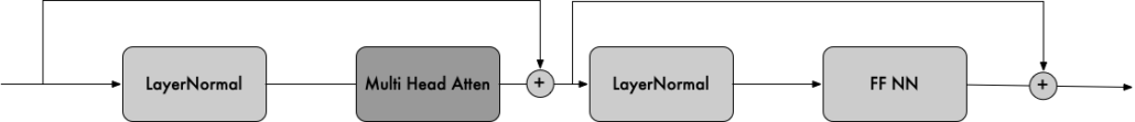
the decoder network’s components are as same as encoder, but the attention layer will be removed by masked attention layer and cross attention layer. (figure-1)

Wolfram

crossAttentionBlock[embedDim_, heads_] := NetInitialize[
  NetGraph[
   FunctionLayer[
    Block[{keys, queries, values, seq},
      seq = 
       NormalizationLayer[2 ;;, "Same", 
         "Epsilon" -> 0.0001 ][#Input];
      keys = NetMapOperator[{heads, embedDim/heads}][seq];
      values = NetMapOperator[{heads, embedDim/heads}][seq];
      queries = NetMapOperator[{heads, embedDim/heads}][ #Query];
      seq = 
       AttentionLayer["Dot", "MultiHead" -> True, 
         "ScoreRescaling" -> "DimensionSqrt"][<|"Key" -> keys, 
         "Query" -> queries, "Value" -> values|>];
      seq = NetMapOperator[embedDim][seq];
      seq = DropoutLayer[0.1][seq];
      seq = #Query + seq
      ] &,
    "Input" -> {"Varying", embedDim},
    "Query" -> {"Varying", embedDim}
    ]
   ]
  ]
Information[crossAttentionBlock[128, 8], "SummaryGraphic"]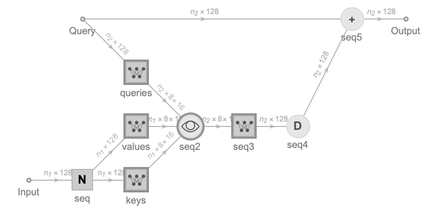

The input socket’s data (Key, Value) of cross attention layer is from output of encoder stack, the query socket’s data (Query) of cross attention layer is from the output of decoder masked attention layer.

Encoder and Decoder Stack

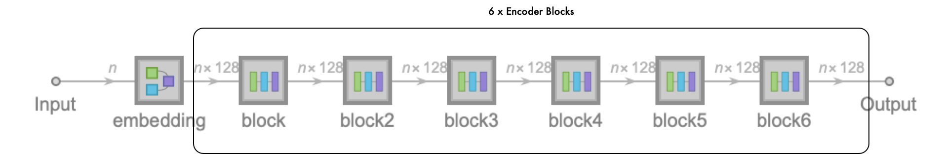
Now we have encoder and decoder block, we can make them stack into new big neural network.

Wolfram

encoderStack[embedDim_, heads_, blocks_Integer, vocabulary_] := 
 Block[
  {emBlock, encoderBlock},
  emBlock = 
   embeddingBlock["depth" -> embedDim, "voca" -> vocabulary, 
    "hardCode" -> False];
  encoderBlock = 
   NetChain[{selfAttentionBlock[embedDim, heads], 
     feedForwardBlock[embedDim]}];
  NetInitialize@NetGraph@FunctionLayer[
     Block[{embedding, block},
       embedding = emBlock[#Input];
       block = encoderBlock[embedding];
       Do[block = encoderBlock[block], {blocks - 1}];
       block
       ] &,
     "Input" -> {"Varying", NetEncoder[{"Class", vocabulary}]}
     ]
  ]
encoderStack[128, 8, 1, voca]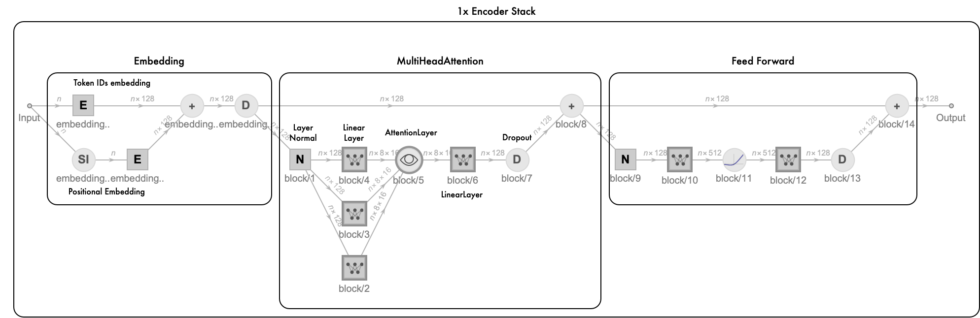

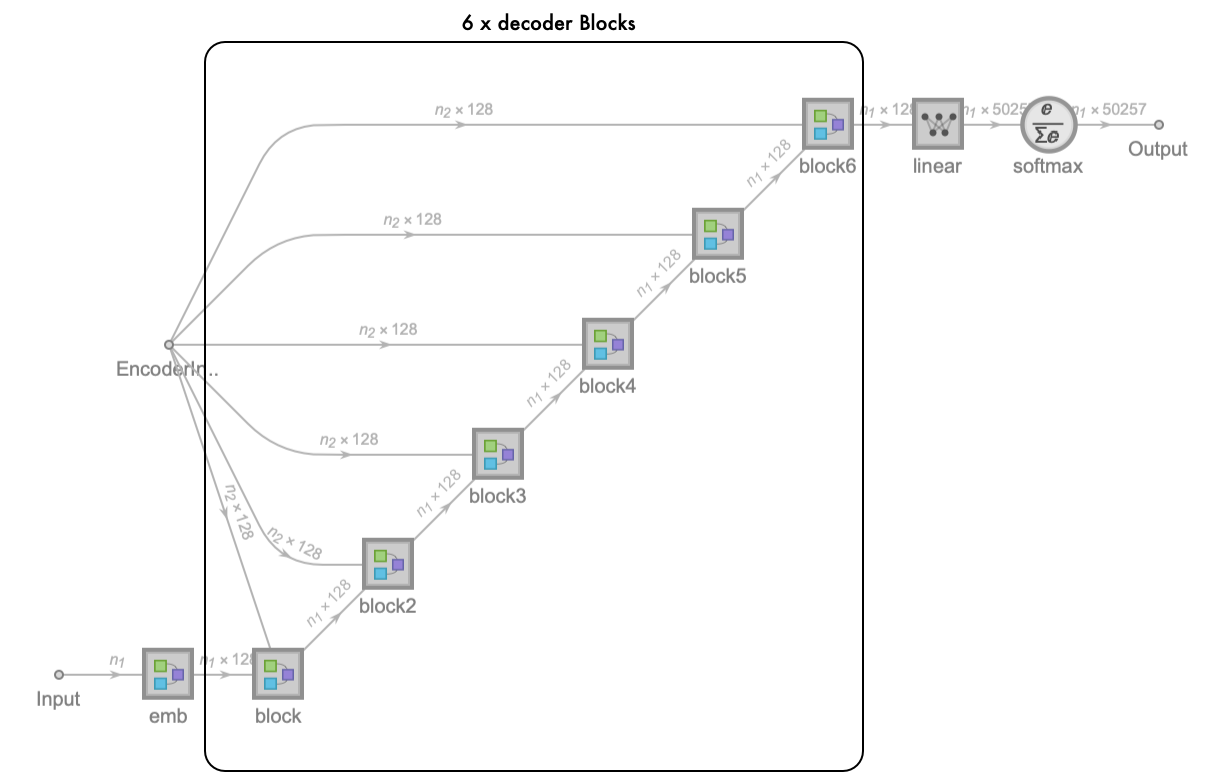
Wolfram

decoderStack[embedDim_, heads_, blocks_Integer, vocabulary_] := 
 Block[
  {emBlock, decoderBlock},
  emBlock = 
   embeddingBlock["depth" -> embedDim, "voca" -> vocabulary, 
    "hardCode" -> False];
  decoderBlock = NetFlatten@NetGraph[
     <|"maskedSelfAtt" -> 
       selfAttentionBlock[embedDim, heads, "Causal"],
      "crossatt" -> crossAttentionBlock[embedDim, heads],
      "FFN" -> feedForwardBlock[embedDim]|>,
     {NetPort["Input"] -> NetPort["maskedSelfAtt", "Input"],
      "maskedSelfAtt" -> NetPort["crossatt", "Query"],
      NetPort["EncoderInput"] -> NetPort["crossatt", "Input"],
      "crossatt" -> "FFN"}
     ];
  NetInitialize@NetGraph@FunctionLayer[
     Block[{emb, block, , linear, softmax},
       emb = emBlock[#Input];
       block = decoderBlock[emb];
       Do[block = decoderBlock[block], {blocks - 1}];
       linear = LinearLayer[] /@ block;
       softmax = SoftmaxLayer[] /@ linear
       ] &,
     "Input" -> {"Varying", NetEncoder[{"Class", vocabulary}]},
     "Output" -> {"Varying", NetDecoder[{"Class", vocabulary}]}
     ]
  ] 
decoderStack[128, 8, 1, voca]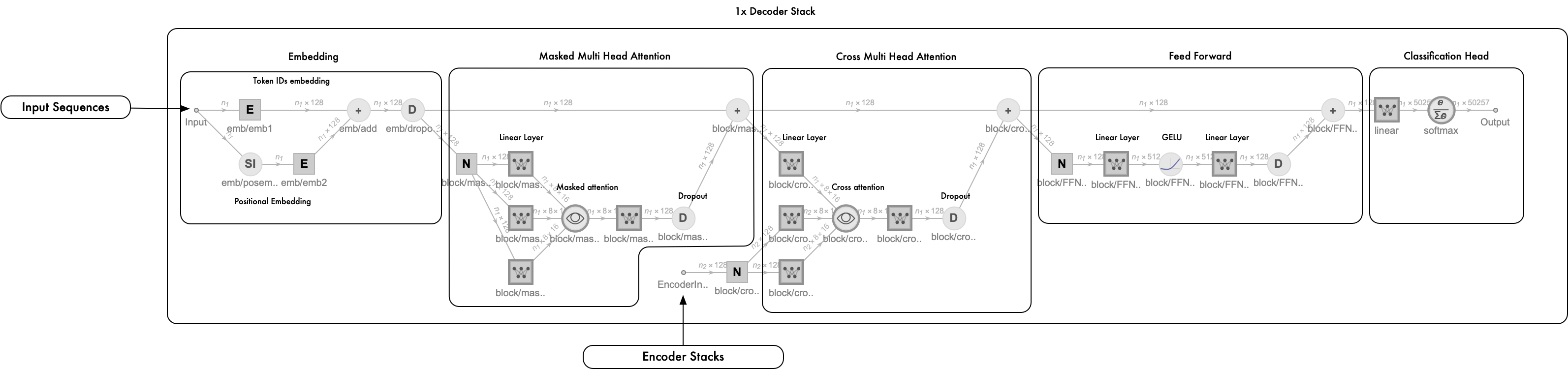

finally we merge the encoder stack and decoder stack (the completed transformer model):

Training Transformer Model

we will training sequence to sequence transformer model to translate sequence from English to French. So how to training seq to seq transformer model?

Training Algorithm:

\text{Input: } \left\{x_n,y_n\right\},\text{a dataset of sequence pairs, dataset size is } N_{\text{data}} \\ \text{Input: $\theta $, initial transformer parameters} \\ \text{Output: } \tilde{\theta } \text{, the trained parameters} \\ \text{for i = 1,2,3 ... } N_{\text{epochs }} \text{do} \\ \text{for n = 1,2,3, ..., } N_{\text{data }} \text{do} \\ \text{$\ell $ $\leftarrow $ } \text{length}\left(y_n\right) \\ \text{P($\theta $) $\leftarrow $ } \text{TransformerNet}\left(x_n\right. \text{, } y_n \text{$|\theta $)} \\ \text{loss($\theta $) = -} \sum _{t=1}^{\ell -1} \text{LogP}(\theta )\left[y_n(t+1),t\right] \\ \theta \leftarrow \theta -\theta \eta \cdot \nabla \text{loss} \\ \text {end for} \\ \text {end for} \\ \text{return } \tilde{\theta } \text{ = $\theta $}

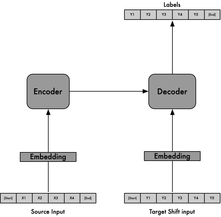
The Algorithm can be explained below diagram: SourceInput is X, Target Input is Y(Left shifted by1), Labels is Y (Right shifted by 1), [start] [end] representation of BOS(begin of sequence), EOS(end of sequence)

Prepare Datasets:

Wolfram

(* Dataset *)
(* please download the database from https://www.manythings.org/anki/ *)
dataFilePath = "~/CineNeural/notebooks/Datasets/fra-eng/fra.txt"
text = Import[dataFilePath];
sentencePairs = Rule @@@ Part[StringSplit[StringSplit[text, "\n"], "\t"], All, {1, 2}];
$randomSeed = 1357;
SeedRandom[$randomSeed];
trainingSet = RandomSample[sentencePairs];

netEncoder = ResourceFunction["GPTTokenizer"][];
netDecoder = NetDecoder[{"Class", NetExtract[ResourceFunction["GPTTokenizer"][], "Tokens"]}]

trainingTokens = MapAt[netEncoder, trainingSet, {All, {1, 2}}];
(* in the training Tokens we use 50257 tokenid as bos and eos *)
trainingTokens = MapAt[Join[{50257}, #1, {50257}] &, trainingTokens, {All, {1, 2}}];

x = Keys[trainingTokens]; (* source input *)
y = Values[trainingTokens]; (* target input *)

create training network:

Wolfram

encoder = encoderStack[128, 8, 6, voca];
decoder = decoderStack[128, 8, 6, voca];
transformerNet = 
 NetGraph@
  FunctionLayer[
   Block[{encode, decode, most, rest}, most = Most[#TargetSequence];
     rest = Rest[#TargetSequence]; 
     encode = encoder[#SourceSequence];
     decode = decoder[<|"Input" -> most, "EncoderInput" -> encode|>];
     CrossEntropyLossLayer["Index"][{decode, rest}]] &, 
   "SourceSequence" -> NetEncoder[{"Class", voca}], 
   "TargetSequence" -> NetEncoder[{"Class", voca}]]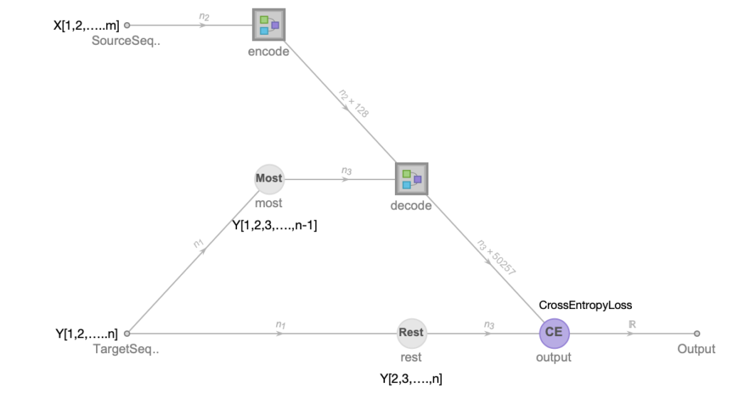

Training Model:

Wolfram

result =
 NetTrain[
  transformerNet, <|"SourceSequence" -> x, "TargetSequence" -> y|>,
  All, MaxTrainingRounds -> 4, ValidationSet -> Scaled[0.1],
  BatchSize -> 16,
  TargetDevice -> {"GPU", All}]

(*save trained model*)
net = result["TrainedNet"]
Export["~/transformer-128depth.wlnet", net]

Inference Transformer Trained Model

seq2seq trained model predicting algorithm:

\text{Input}: \text{A seq2seq transformer and trained parameters } \tilde{\theta } \text { of transformer} \\ \text{Input: x $\in $ } V^* \text{, input sequence} \\ \text{Output: } \tilde{x} \text{ $\in $ } V^* \text{, output sequence} \\ \text{Hyperparameters: $\tau $ $\in $ (0, $\infty $)} \\ \tilde{x} \text{ $\leftarrow $ [bos$\_$token]} \\ y\leftarrow 0 \\ \text{while } y\neq \text{eos$\_$token} \text{ do} \\ \text{P $\leftarrow $ TransformerNet(x, } \tilde{x} \text{ $|$ } \tilde{\theta } ) \\ \text{p $\leftarrow $ P[All, } \text{length}\left(\tilde{x}\right) ] \\ \text{sample a token y from q $\propto $ } p^{1/\tau } \\ \tilde{x} \text{ $\leftarrow $ } \left[\tilde{x}\right. \text{, y]} \\ \text {end} \\ \text{return} \tilde{x}

Wolfram

trainedNet = 
 Import["/Users/alexchen/CineNeural/neural-models/transformer/\
transformer-v2-128depth.wlnet"]

trainedEncodeNet = NetExtract[trainedNet, "encode"]
trainedDecodeNet = NetExtract[trainedNet, "decode"]
predictor = 
 NetReplacePart[
  trainedDecodeNet, {"Output" -> NetDecoder[{"Class", voca}]}]


translate[sourceSentence_String] := 
 Module[{sourceSequence, translationSequence, translationTokens, 
   tokenEncoder, tokenDecoder},
   
  sourceSequence = 
   trainedEncodeNet[
    Join[{50257}, netEncoder[sourceSentence], {50257}]]; (* add bos and eos for source sequence *)
    
  tokenEncoder = NetEncoder[{"Class", voca}];
  tokenDecoder = 
   NetDecoder[{"Class", 
     NetExtract[ResourceFunction["GPTTokenizer"][], "Tokens"]}];
     
  translationSequence = NestWhile[
    Append[
      #,
      tokenEncoder[Last[predictor[<|
          "Input" -> #,
          "EncoderInput" -> sourceSequence|>]]]] &,
    {50257},
    (* check last token of the sequence, if not eos token, then append to sequence for next prediction. *)
    If[Length@# >= 2, Last[#] != 50257, True] &,
    1, 512];
  translationTokens = 
   Map[tokenDecoder[UnitVector[Length@voca, #]] &, 
    translationSequence];
    
  StringReplace[StringJoin[Cases[translationTokens, _String]], 
   "Ġ" -> " "]
  ]

translate["thank you"] (* return Franch: Merci. *)