Kinematic model of Mecanum wheel
What is Mecanum wheel
The mecanum wheel is an omnidirectional wheel design for a land based vehicle and invented by Swedish Engineer – Bengt Erland Ilon.
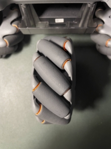
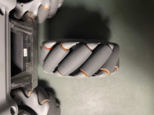
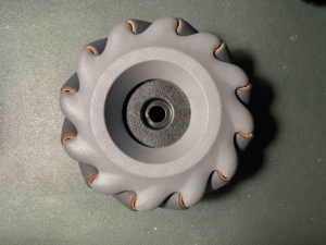
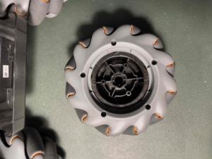
There are a series of free moving rollers attached to the whole circumference of vehicle’s wheel, these rollers typically have a 45 degree to the axle line, and freely about axes in the plane of the wheel, but the overall side profile of the wheel is circular. How the Mecanum wheel drives the mobile robot?
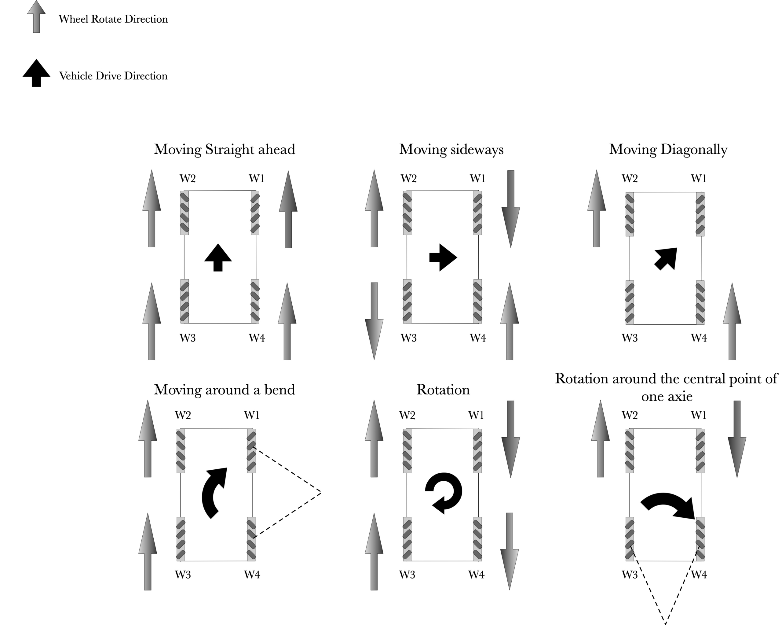
First we will define the wheels sequences:
- FrontRightWheel as w1
- FrontLeftWheel as w2
- RearLeftWheel as w3
- RearRightWheel as w4
How the vehicle moves:
- Running all four wheels in the same direction and same speed will result moving the vehicle in a forward or backward.
- Running both wheels on one side in one direction and other side in the opposite direction, will result in a static rotation of the vehicle.
- Running w1 backward, w2 forward, w3 backward, w4 forward, the result of vehicle will moving to right sideway.
- Running w2 forward, w4 forward and stop other wheels, the result of vehicle will moving to top-right diagonally.
- Running w2 and w3 forward, and stop other wheels, the result of vehicle will moving rotate around the point on x-axies.
- Running w2 forward and w1 backward, and stop other wheels, the result of vehicle will moving rotate around the point on y-axies.
Question:
How the wheel speed map to the mobile robot velocity, if we know robot’s velocity is:
\left\{v_x,v_y,\omega _z\right\}
\\
v_x,
v_y
\text{ - }
\text{robot linear} \text{ velocity} \\
\omega _z
\text{ - }
\text{robot angular} \text{ velocity}
what is the wheels angular velocity need?
solve this map problem, we need to use kinematic model.
Kinematic model
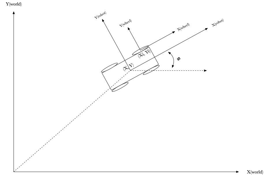
Define
- XY – world: inertial frame, call it frame A
- XY – robot: robot’s base frame, call it frame C
- XY – wheel: robot’s wheel base frame as frame B, and wheels center point at {xi, yi) in Frame C
- Robot’s position is (x,y) in Frame A, and it’s orientation angle is 𝜙
- v-x, v-y are wheel’s linear velocity, v-slide is sliding speed, v-drive is direction drive speed.
- free sliding direction angle with the Frame B -y axes is 𝛾.
- frame B (wheel) angle with frame C(robot) is 𝛽.
- 𝜔 – wheel’s angular velocity.
- v-c is robot’s linear velocity in Frame C, v-a is robot’s linear velocity in Frame A.
- 𝜔i – robot’s i-th wheel
- x,y – the distances from the vehicle robot geometric centers to the axis of the wheels geometric centers.
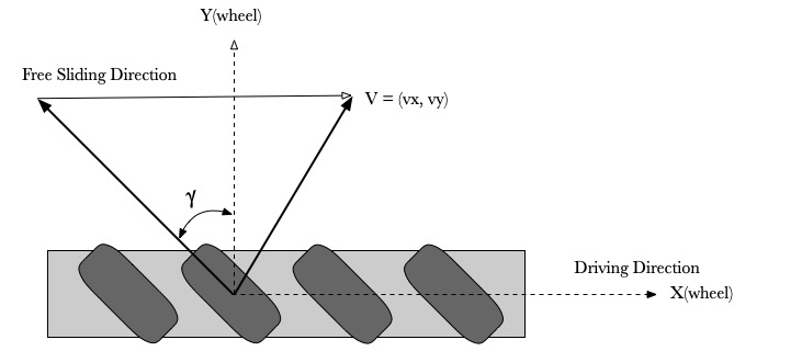
v_{\text{drive}}=v_x+\tan (\gamma ) v_y \\
v_{\text{slide}}=\frac{v_y}{\cos (\gamma )}
\left(
\begin{array}{c}
v_x \\
v_y \\
\end{array}
\right)=\left(
\begin{array}{c}
1 \\
0 \\
\end{array}
\right) v_{\text{drive}}+v_{\text{slide}} \left(
\begin{array}{c}
-\sin (\gamma ) \\
\cos (\gamma ) \\
\end{array}
\right)\omega =\frac{v_{\text{driver}}}{r}=\frac{v_x+\tan (\gamma ) v_y}{r}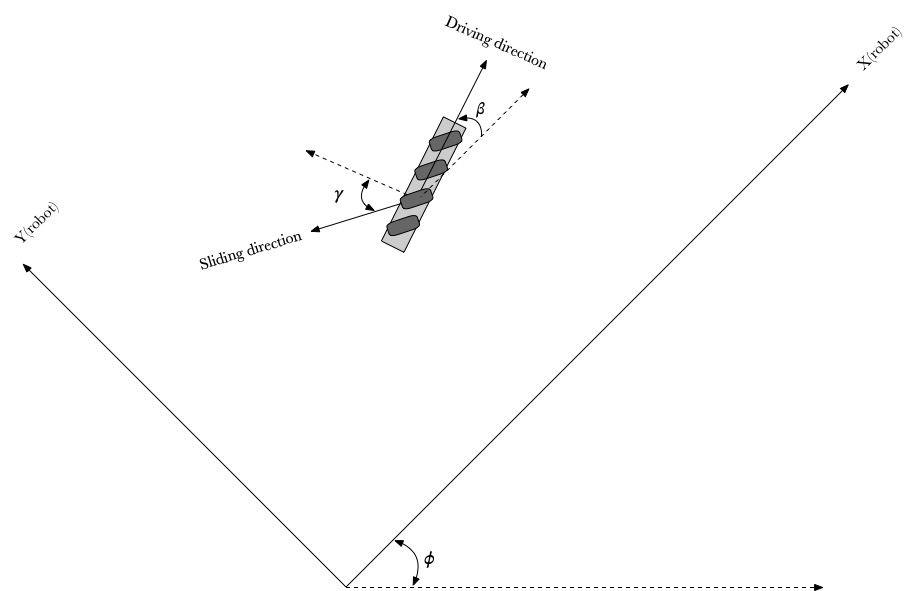
v_a=\left(
\begin{array}{c}
 \dot{\phi } \\
 \dot{x} \\
 \dot{y} \\
\end{array}
\right)=\left(
\begin{array}{ccc}
 1 & 0 & 0 \\
 0 & \cos (\phi ) & -\sin (\phi ) \\
 0 & \sin (\phi ) & \cos (\phi ) \\
\end{array}
\right).\left(
\begin{array}{c}
 \omega _{\text{cz}} \\
 v_{\text{cx}} \\
 v_{\text{cy}} \\
\end{array}
\right)
v_c=\left(
\begin{array}{c}
 \omega _{\text{cz}} \\
 v_{\text{cx}} \\
 v_{\text{cy}} \\
\end{array}
\right)=\left(
\begin{array}{ccc}
 1 & 0 & 0 \\
 0 & \cos (\phi ) & \sin (\phi ) \\
 0 & -\sin (\phi ) & \cos (\phi ) \\
\end{array}
\right).\left(
\begin{array}{c}
 \frac{d\phi }{dt} \\
 \frac{dx}{dt} \\
 \frac{dy}{dt} \\
\end{array}
\right)=\left(
\begin{array}{ccc}
 1 & 0 & 0 \\
 0 & \cos (\phi ) & \sin (\phi ) \\
 0 & -\sin (\phi ) & \cos (\phi ) \\
\end{array}
\right).\left(
\begin{array}{c}
 \dot{\phi } \\
 \dot{x} \\
 \dot{y} \\
\end{array}
\right)
Inverse Kinematic
we can decompose linear velocity on Frame A (world) to Frame C(robot), then to Frame B(wheel), so we get:
Transform Matrix
Transfer v-a to v-c
T_1=\left(
\begin{array}{ccc}
 1 & 0 & 0 \\
 0 & \cos (\phi ) & \sin (\phi ) \\
 0 & -\sin (\phi ) & \cos (\phi ) \\
\end{array}
\right).\left(
\begin{array}{c}
 \dot{\phi } \\
 \dot{x} \\
 \dot{y} \\
\end{array}
\right)
Transfer v-c to v-x, v-y in wheel frame B
Because our vehicle mobile robot can both translational and rotational movements, so the angular velocity also need to projection of linear velocity of wheel.
T_1=\left\{\dot{\phi },\dot{x} \cos (\phi )+\dot{y} \sin (\phi ),\dot{y} \cos (\phi )-\dot{x} \sin (\phi )\right\}\omega _{\text{robot}}=\dot{\phi } \\
v_{\text{xRobot}}=\dot{x} \cos (\phi )+\dot{y} \sin (\phi ) \\
v_{\text{yRobot}}=\dot{y} \cos (\phi )-\dot{x} \sin (\phi )v_{\text{xwheel}}=v_{\text{xRobot}}-\sin (\beta ) \omega _{\text{robot}} \sqrt{x_i^2+y_i^2}=v_{\text{xRobot}}-\frac{y_i \omega _{\text{robot}} \sqrt{x_i^2+y_i^2}}{\sqrt{x_i^2+y_i^2}}=v_{\text{xRobot}}-\dot{\phi } y_i \\
v_{\text{ywheel}}=\cos (\beta ) \omega _{\text{robot}} \sqrt{x_i^2+y_i^2}+v_{\text{yrobot}}=x_i \omega _{\text{robot}} \sqrt{x_i^2+y_i^2}+v_{\text{yrobot}}=\dot{\phi } x_i+v_{\text{yrobot}}So, get the translational matrix from robot frame to wheel frame
T_2=\left(
\begin{array}{ccc}
 -y_i & 1 & 0 \\
 x_i & 0 & 1 \\
\end{array}
\right).T_1
then, get the rotational matrix from robot frame to wheel frame
T_3=\left(
\begin{array}{cc}
 \cos \left(\beta _i\right) & \sin \left(\beta _i\right) \\
 -\sin \left(\beta _i\right) & \cos \left(\beta _i\right) \\
\end{array}
\right).T_2
Transfer v-x, v-y to wheel’s angular speed
T_4=\left(
\begin{array}{cc}
 \frac{1}{r_i} & \frac{\tan \left(\gamma _i\right)}{r_i} \\
\end{array}
\right).T_3
finally, we get the wheel’s angular velocity
\omega _i=T_1.T_2.T_3.T_4.\left(
\begin{array}{c}
 \dot{\phi } \\
 \dot{x} \\
 \dot{y} \\
\end{array}
\right)
\omega _i=\left(
\begin{array}{cc}
\frac{1}{r_i} & \frac{\tan \left(\gamma _i\right)}{r_i} \\
\end{array}
\right).\left(
\begin{array}{cc}
\cos \left(\beta _i\right) & \sin \left(\beta _i\right) \\
-\sin \left(\beta _i\right) & \cos \left(\beta _i\right) \\
\end{array}
\right).\left(
\begin{array}{ccc}
-y_i & 1 & 0 \\
x_i & 0 & 1 \\
\end{array}
\right).\left(
\begin{array}{ccc}
1 & 0 & 0 \\
0 & \cos (\phi ) & \sin (\phi ) \\
0 & -\sin (\phi ) & \cos (\phi ) \\
\end{array}
\right).\left(
\begin{array}{c}
\dot{\phi } \\
\dot{x} \\
\dot{y} \\
\end{array}
\right)\omega _i=h_i(\phi ).\left(
\begin{array}{c}
\dot{\phi } \\
\dot{x} \\
\dot{y} \\
\end{array}
\right)h_i(\phi )=\left(
\begin{array}{ccc}
\frac{\sec \left(\gamma _i\right) \left(x_i \sin \left(\beta _i+\gamma _i\right)-y_i \cos \left(\beta _i+\gamma _i\right)\right)}{r_i} & \frac{\sec \left(\gamma _i\right) \cos \left(\beta _i+\gamma _i+\phi \right)}{r_i} & \frac{\sec \left(\gamma _i\right) \sin \left(\beta _i+\gamma _i+\phi \right)}{r_i} \\
\end{array}
\right)specially, when the 𝛟 is 0:
h_i(0)=\left(
\begin{array}{ccc}
 \frac{\sec \left(\gamma _i\right) \left(x_i \sin \left(\beta _i+\gamma _i\right)-y_i \cos \left(\beta _i+\gamma _i\right)\right)}{r_i} & \frac{\sec \left(\gamma _i\right) \cos \left(\beta _i+\gamma _i\right)}{r_i} & \frac{\sec \left(\gamma _i\right) \sin \left(\beta _i+\gamma _i\right)}{r_i} \\
\end{array}
\right)
Assume our vehicle robot have four wheels, we get H Matrix:
H=\left(
\begin{array}{c}
 h_1(\phi ) \\
 h_2(\phi ) \\
 h_3(\phi ) \\
 h_4(\phi ) \\
\end{array}
\right)
now, we consider the angular of robot’s frame with robot wheel’s frame 𝛽 is 0, and set W1, W2, W3, W4 value, “->” means substitute the symbol value of the formula.
W_1=\left\{\gamma _1\to \frac{\pi }{4},\beta _1\to 0,x_1\to x,y_1\to -y,r_1\to r\right\}\\
W_2=\left\{\gamma _2\to -\frac{\pi }{4},\beta _2\to 0,x_2\to x,y_2\to y,r_2\to r\right\} \\
W_3=\left\{\gamma _3\to \frac{\pi }{4},\beta _3\to 0,x_3\to -x,y_3\to y,r_3\to r\right\} \\
W_4=\left\{\gamma _4\to -\frac{\pi }{4},\beta _4\to 0,x_4\to -x,y_4\to -y,r_4\to r\right\}
define x + y = l, we get the inverse kinematic:
\left(
\begin{array}{c}
 \omega _1 \\
 \omega _2 \\
 \omega _3 \\
 \omega _4 \\
\end{array}
\right)=\left(
\begin{array}{c}
 \frac{v_{\text{xRobot}}+v_{\text{yRobot}}+(x+y) \omega _{\text{zRobot}}}{r} \\
 \frac{v_{\text{xRobot}}-v_{\text{yRobot}}-(x+y) \omega _{\text{zRobot}}}{r} \\
 \frac{v_{\text{xRobot}}+v_{\text{yRobot}}-(x+y) \omega _{\text{zRobot}}}{r} \\
 \frac{v_{\text{xRobot}}-v_{\text{yRobot}}+(x+y) \omega _{\text{zRobot}}}{r} \\
\end{array}
\right)=\frac{1}{r}.\left(
\begin{array}{ccc}
 1 & 1 & l \\
 1 & -1 & -l \\
 1 & 1 & -l \\
 1 & -1 & l \\
\end{array}
\right).\left(
\begin{array}{c}
 \dot{x} \\
 \dot{y} \\
 \dot{\phi } \\
\end{array}
\right)
Forward Kinematic
we know the inverse kinematic, so it’s very easy to let us compute the forward kinematic through inverse matrix operation.
T=H(0)
\omega =T.\left(
\begin{array}{c}
 \dot{\phi } \\
 \dot{x} \\
 \dot{y} \\
\end{array}
\right)
T=\left(
\begin{array}{ccc}
\frac{l}{r} & \frac{1}{r} & \frac{1}{r} \\
-\frac{l}{r} & \frac{1}{r} & -\frac{1}{r} \\
-\frac{l}{r} & \frac{1}{r} & \frac{1}{r} \\
\frac{l}{r} & \frac{1}{r} & -\frac{1}{r} \\
\end{array}
\right)=\frac{1}{r}.\left(
\begin{array}{ccc}
l & 1 & 1 \\
-l & 1 & -1 \\
-l & 1 & 1 \\
l & 1 & -1 \\
\end{array}
\right)T^{-1}.\omega =\left(
\begin{array}{c}
\dot{x} \\
\dot{y} \\
\dot{\phi } \\
\end{array}
\right)T^{-1}=\left(T^T.T\right)^{-1}.T^TT^{-1}=\left(
\begin{array}{cccc}
\frac{r}{4 l} & -\frac{r}{4 l} & -\frac{r}{4 l} & \frac{r}{4 l} \\
\frac{r}{4} & \frac{r}{4} & \frac{r}{4} & \frac{r}{4} \\
\frac{r}{4} & -\frac{r}{4} & \frac{r}{4} & -\frac{r}{4} \\
\end{array}
\right)T^{-1}=\left(
\begin{array}{cccc}
\frac{r}{4 l} & -\frac{r}{4 l} & -\frac{r}{4 l} & \frac{r}{4 l} \\
\frac{r}{4} & \frac{r}{4} & \frac{r}{4} & \frac{r}{4} \\
\frac{r}{4} & -\frac{r}{4} & \frac{r}{4} & -\frac{r}{4} \\
\end{array}
\right)=\frac{r}{4}.\left(
\begin{array}{cccc}
\frac{1}{l} & -\frac{1}{l} & -\frac{1}{l} & \frac{1}{l} \\
1 & 1 & 1 & 1 \\
1 & -1 & 1 & -1 \\
\end{array}
\right)finally, we get the forward kinematic:
\left(
\begin{array}{c}
 \dot{\phi } \\
 \dot{x} \\
 \dot{y} \\
\end{array}
\right)=\frac{r}{4}.\left(
\begin{array}{cccc}
 \frac{1}{l} & -\frac{1}{l} & -\frac{1}{l} & \frac{1}{l} \\
 1 & 1 & 1 & 1 \\
 1 & -1 & 1 & -1 \\
\end{array}
\right).\left(
\begin{array}{c}
 \omega _1 \\
 \omega _2 \\
 \omega _3 \\
 \omega _4 \\
\end{array}
\right)
Conclusion
Through this article, we get the forward kinematic (FK) and inverse kinematic (IK) of Mecanum wheels. Using the FK and IK, we can more controllable to drive our robot which using mecanum wheel.
Robot’s Mecanum wheels parameters:
| wheel id | wheels Name | 𝛾 | 𝛽 | X | Y | R |
| 1 | FrontRight (FR) | 𝜋/4 | 0 | x | -y | r |
| 2 | FrontLeft (FL) | -𝜋/4 | 0 | x | y | r |
| 3 | RearLeft (RL) | 𝜋/4 | 0 | -x | y | r |
| 4 | RearRight (RR) | -𝜋/4 | 0 | -x | -y | r |
Forward Kinematic
\left(
\begin{array}{c}
 \dot{\phi } \\
 \dot{x} \\
 \dot{y} \\
\end{array}
\right)=\frac{r}{4}.\left(
\begin{array}{cccc}
 \frac{1}{l} & -\frac{1}{l} & -\frac{1}{l} & \frac{1}{l} \\
 1 & 1 & 1 & 1 \\
 1 & -1 & 1 & -1 \\
\end{array}
\right).\left(
\begin{array}{c}
 \omega _1 \\
 \omega _2 \\
 \omega _3 \\
 \omega _4 \\
\end{array}
\right)
Inverse Kinematic
\left(
\begin{array}{c}
 \omega _1 \\
 \omega _2 \\
 \omega _3 \\
 \omega _4 \\
\end{array}
\right)=\frac{1}{r}.\left(
\begin{array}{ccc}
 l & 1 & 1 \\
 -l & 1 & -1 \\
 -l & 1 & 1 \\
 l & 1 & -1 \\
\end{array}
\right).\left(
\begin{array}{c}
 \dot{\phi } \\
 \dot{x} \\
 \dot{y} \\
\end{array}
\right)
Leave a Reply
Want to join the discussion?Feel free to contribute!